
Introduction
Each year, fires blaze across the African continent, impacting ecosystems, air quality, and communities. Some fires are beneficial and part of natural cycles, while others—especially wildfires—cause significant damage and release vast amounts of CO₂ and pollutants into the atmosphere. This project aimed to develop a machine-learning model to predict wildfire burn areas across Zimbabwe, allowing for better preparedness and resource allocation. The prediction model was built on data from 2001 to 2013, using environmental and climatic factors, to forecast burn areas for 2014-2016.
Table of Contents
- 1. Overview and Objectives
- 2. Architecture Diagram
- 3. ETL Process
- 4. Data Modeling
- 5. Inference
- 6. Performance Metrics
- 7. Error Handling and Logging
- 8. Final Notes
- 9. Conclusion
- Final Ranking
1. Overview and OBJECTIVES
High-Level Description
This project addresses the problem of predicting wildfire burn areas based on various environmental and climatic factors. The solution leverages machine learning, specifically the LightGBM algorithm, to model and predict the target variable, which is the percentage of the area burned by wildfires.
Objectives and Expected Outcomes
The main objective is to create an accurate predictive model that can be used by stakeholders to forecast wildfire impacts, potentially aiding in preventive measures and resource allocation. The expected outcome is a well-generalized model that performs consistently across both the public and private leaderboards.
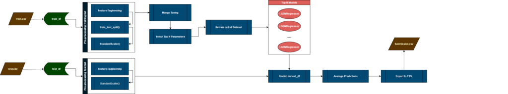
2. Architecture diagram
Below is the architecture diagram that illustrates the entire data flow and components, from ETL to modeling and inference:
3. etl process
Extract
The data used for this solution was provided in CSV format and consisted of three files:
- Train.csv: This is the training dataset with a shape of (83148 rows, 29 columns). It contains various features related to climatic variables, land cover types, and other relevant data.
- Test.csv: This is the test dataset with a shape of (25584 rows, 29 columns). Similar to the training set, it contains the same features but without the target variable « burn_area ».
- variable_definitions.csv: This file acts as a data dictionary, providing detailed descriptions and definitions for each feature in the datasets.
The data is structured in a tabular format with a mixture of continuous and categorical variables. The CSV files were read into the environment using the pandas library, specifically utilizing the pd.read_csv() function. This method efficiently handles the data extraction, ensuring that all features are correctly loaded into dataframes for subsequent processing.
Considerations were given to the data volume and the frequency of extraction. The datasets are of a manageable size, allowing for quick and efficient data loading. The data was static and provided as part of the competition, with no need for periodic updates or frequent extraction.
# import Pandas
import pandas as pd

# Display option to see the whole description for each variable
pd.set_option('display.max_colwidth', None)

# The data dictionary
var_defs = pd.read_csv('variable_definitions.csv')

# The training data

train = pd.read_csv('Train.csv')

# The test set
test = pd.read_csv('Test.csv')
test["burn_area"] = 1 # used later in feature engineering, to avoid No such column error
Transform
The data underwent several preprocessing and feature engineering steps, including:
- Date Features: Extracted from the ‘ID’ column (e.g., year, month, day, day of the year, season).
- Interaction Terms: Created interactions between temperature and precipitation.
- Rolling Statistics: Applied rolling mean and standard deviation on the temperature data.
- Lagged Variables: Generated lagged features for climate data.
- Binary Flags: Created binary indicators for the presence of various land cover types.
- Dominant Land Type: Identified the dominant land cover type.
- Drought Indicator: Added a binary indicator for drought conditions.
- Adjusted Temperature: Computed temperature adjusted for elevation.
- Water Balance: Derived from precipitation and runoff data.
- Log Transformation: Applied to the target variable, burn_area, to normalize the distribution.
# processing function for feature engineering
def fe_process(train):
    # Deep copy the dataframe to avoid data loss
    df = train.copy(deep=True)

    # Split the ID (eg 127_2017-01-03) to get the date string, which we convert to datetime to make life easier
    df['date'] = pd.to_datetime(train['ID'].apply(lambda x: x.split('_'[1]))

    # Extracting date-related features
    df['year'] = df['date'].dt.year
    df['month'] = df['date'].dt.month
    df['day'] = df['date'].dt.day
    df['day_of_year'] = df['date'].dt.dayofyear
    df['season'] = df['month'] % 12 // 3 + 1 # 1: Winter, 2: Spring, 3: Summer, 4: Fall

    # Interaction terms for climate variables
    df['temp_precip_interaction'] = df['climate_tmmx'] * df['climate_pr']
    df['hot_and_dry'] = df['climate_tmmx'] / (df['climate_pr'] + 1)

    # Rolling statistics for climate variables
    df['climate_tmmx_rolling_mean_3'] = df['climate_tmmx'].rolling(window=3).mean()
    df['climate_tmmx_rolling_std_3'] = df['climate_tmmx'].rolling(window=3).std()

    # Lagged variables
    df['climate_pr_lag1'] = df['climate_pr'].shift(1)
    df['climate_tmmx_lag1'] = df['climate_tmmx'].shift(1)

    # Binary flags for landcover types
    landcover_cols = [f'landcover_{i}' for i in range(9)]
    for col in landcover_cols:
        df[f'has_{col}'] = (df[col] > 0).astype(int)

    # Dominant land type
    df['dominant_land_type'] = df[landcover_cols].idxmax(axis=1)
    df['dominant_land_type'] = df['dominant_land_type'].str.extract('(\d+)', expand=False).astype(int)

    # Drought indicator
    df['is_drought'] = (df['climate_pdsi'] < -2).astype(int)

    # Elevation adjusted temperature
    df['adjusted_tmmx'] = df['climate_tmmx'] - (0.0065 * df['elevation'])

    # Water balance
    df['water_balance'] = df['climate_pr'] - df['climate_ro']

    # Log transformation of the target variable to adress skewness
    df['log_burn_area'] = np.log1p(df['burn_area'])

    # Fill NA values created by rolling statistics and lagged variables
    df = df.apply(lambda x: x.bfill(), axis=0)

    # Dropping redundant and unnecessary columns
    columns_to_drop = ['date', 'day', 'climate_tmmx', 'climate_tmmn', 'climate_vap', 'climate_swe', 'climate_pr', 'climate_ro']
    columns_to_drop.extend(landcover_cols)
    df.drop(columns_to_drop, axis=1, inplace=True)

    return df
Load
The transformed data was used directly in memory within the Jupyter notebook environment. No additional data storage or indexing strategies were applied
4. data modeling
Description of Data Models and Training Process
- Model Used: The solution uses the LightGBM regressor (LGBMRegressor), known for its efficiency and scalability in handling large datasets with high-dimensional data.
- Feature Engineering: Extensive feature engineering was applied as described in the ETL section. The features were then standardized using StandardScaler where necessary.
- Hyperparameter Tuning: Mango, a parallel hyperparameter tuning library was utilized to tune hyperparameters. Parameters such as learning rate, number of leaves, and boosting rounds were fine-tuned using its Bayesian optimization.
- Training: The dataset was split into training and validation sets using train_test_split, and the model was trained using the LightGBM framework.
- Evaluation: The model’s performance was evaluated using Root Mean Squared Error (RMSE), a standard metric for regression tasks.
Model Training
The model training phase involves using Mango to optimize the hyperparameters for the LightGBM Regressor (LGBMRegressor). In this phase, the objective_function is employed to assess different hyperparameter configurations. The function initializes the LightGBM model with the specified parameters, trains it on the scaled training data, and evaluates its performance on the validation set. The performance is measured using Root Mean Squared Error (RMSE), and this error metric is collected for each configuration to determine which set of parameters performs best. The goal is to find the most effective hyperparameters that yield the lowest RMSE, thereby improving the model’s predictive accuracy.
The early_stopping_function is employed to terminate the optimization early if certain criteria are met. It monitors RMSE values and stops the process if the RMSE falls below a specified target threshold (0.018) or if no significant improvement is observed over a set number of iterations. This ensures efficient use of computational resources by preventing unnecessary calculations once optimal performance is achieved.
The param_space defines the range of hyperparameters to be explored, including learning rate, number of leaves, maximum depth, and other parameters specific to LightGBM. These ranges are selected to balance between a thorough search and computational efficiency. Finally, the conf_dict specifies the configuration for the Mango optimization library, including domain size, number of iterations, and batch size, allowing for a detailed and parallel evaluation of hyperparameter settings while utilizing early stopping to enhance optimization efficiency.
# Define the objective function
def objective_function(param_list):
    results = []

    for params in param_list:
        # Convert integer parameters to the appropriate type
        params['num_leaves'] = int(params['num_leaves'])
        params['max_depth'] = int(params['max_depth']) if params.get('max_depth') is not None else None
        params['min_data_in_leaf'] = int(params['min_data_in_leaf'])
        params['bagging_freq'] = int(params['bagging_freq'])
        params['max_bin'] = int(params['max_bin'])
        params['min_child_weight'] = float(params['min_child_weight'])

        # Initialize the model with the current hyperparameters
        model = LGBMRegressor(**params, verbosity= -1)

        # Fit the model on the training data
        model.fit(X_train_scaled, y_train)

        # Predict on the validation data
        y_pred = model.predict(X_valid_scaled)

        # Calculate RMSE
        rmse = np.sqrt(mean_squared_error(y_valid, y_pred))

        # Append the result to the results list
        results.append(rmse)

    return results


# Define the early stopping function
def early_stopping_function(results):
    patience = 10  # Number of iterations to wait for improvement
    min_improvement = 0.0001  # Minimum change to be considered an improvement
    target_rmse = 0.018  # Stop if RMSE falls below this threshold

    best_rmse = results['best_objective']
    objective_values = results['objective_values']

    # Stop if the best RMSE is below the target RMSE
    if best_rmse < target_rmse:
        print("Early stopping: RMSE below target threshold.")
        return True

    # Stop if no improvement over the last `patience` iterations
    if len(objective_values) > patience:
        recent_values = objective_values[ - patience:]
        if all(abs(val - best_rmse) < min_improvement for val in recent_values):
            print("Early stopping: No improvement over the last {} iterations.".format(patience))
            return True

    # Continue optimization if none of the conditions are met
    return False


# Define the hyperparameter space
param_space = {
    'learning_rate': (0.01, 0.2),  # Narrowed range for more effective search
    'num_leaves': (20, 200),  # Extended range for deeper trees
    'max_depth': (3, 15),  # Extended depth for more complex models
    'min_data_in_leaf': (5, 100),  # Wider range for fine-tuning regularization
    'feature_fraction': (0.4, 0.9),  # Adjusted for a broader search in feature space
    'bagging_fraction': (0.5, 0.9),  # Focused on strong but not extreme subsampling
    'bagging_freq': (1, 20),  # Wider range for more flexibility in subsampling frequency
    'lambda_l1': (0, 10),  # Increased range for stronger L1 regularization if needed
    'lambda_l2': (0, 10),  # Increased range for stronger L2 regularization if needed
    'min_gain_to_split': (0, 0.5),  # Threshold for splitting nodes
    'max_bin': (200, 500),  # Adjusting number of bins for feature quantization
    'min_child_weight': (1e - 3, 10)  # Minimum sum of instance weight needed in a child
}

# Define the Mango configuration
conf_dict = dict(
    'domain_size'=15000,  # Large domain size for thorough exploration
    'initial_random'=10,  # Initial broad exploration
    'num_iteration'=1000,  # Enough iterations for detailed search
    'batch_size'=10,  # Evaluate multiple configurations in parallel
    'early_stopping'=early_stopping_function
)
Then, the process of tuning hyperparameters using the Mango library can be started. First, a Tuner object is created, initialized with the hyperparameter space (param_space), the objective function (objective_function), and the configuration dictionary (conf_dict).
The tuner.minimize() method is then executed to start the tuning process. This function performs the optimization, evaluating different configurations and identifying the one that minimizes the objective function, which in this case is the Root Mean Squared Error (RMSE).
After the tuning process is complete, the best hyperparameters and their corresponding RMSEs are stored in the results dictionary. The results[‘best_params’] provides the optimal set of hyperparameters, while results[‘best_objective’] gives the lowest RMSE achieved with these parameters.
# Mango Tuner
tuner = Tuner(param_space, objective_function, conf_dict)

# Run the tuning
results = tuner.minimize()

# Best parameters and RMSE
print('Best parameters:', results['best_params'])
print('Best RMSE:', results['best_objective'])
Model Validation
1. Overview of Model Validation
Model validation is a crucial step in the machine learning pipeline to ensure that the model performs well not only on the training data but also on unseen data. This process involves assessing the model’s performance on a separate validation set and selecting the best model based on specific metrics, such as RMSE (Root Mean Squared Error). In our project, the validation process involves multiple steps including hyperparameter tuning using the Mango Tuner, early stopping criteria, and evaluation on the validation dataset.
2. Train/Validation Split
Purpose: The data is split into training and validation sets to ensure that the model does not overfit to the training data. The validation set serves as a proxy for unseen data, allowing us to evaluate how
well the model might perform in real-world scenarios.
Implementation: The original dataset was split into features (X) and the target variable (y). Using the train_test_split function, 80% of the data was allocated to the training set (X_train, y_train), and 20% to the validation set (X_valid, y_valid). The split is performed with a fixed random seed (random_state=666) to ensure reproducibility.
X_train, X_valid, y_train, y_valid = train_test_split(X, y, test_size=0.2, random_state=666)
3. Data Scaling
Purpose: Scaling is necessary to standardize the features, ensuring that each feature contributes equally to the model training process. This is especially important for models that rely on gradient
descent, such as LGBMRegressor.
Implementation: The StandardScaler was used to fit the training data (X_train_scaled) and then transform both the training and validation sets. The same scaler was applied to both sets to ensure consistency.
scaler = StandardScaler()
X_train_scaled = scaler.fit_transform(X_train)
X_valid_scaled = scaler.transform(X_valid)
4. Evaluation of Model Performance
Purpose: After tuning, the model’s performance was evaluated based on the RMSE values obtained during the validation process. The best model was selected based on the lowest RMSE.
Implementation: The best parameters and corresponding RMSE were extracted and reported. Additionally, the top n models were displayed, providing insight into how different hyperparameters affect
model performance.
print('Best parameters:', results['best_params'])
print('Best RMSE:', results['best_objective'])
The top models were sorted by their RMSE values and displayed to show the effectiveness of different hyperparameter configurations.
sorted_results = sorted(all_results, key=lambda x: x[1])

n = 10
print(f"Top {n} models:")
for i, (params, rmse) in enumerate(sorted_results[:n]):
    print(f"Model {i+1}:")
    print(f"RMSE: {rmse}\n")
The model validation process effectively identified the best model configuration, ensuring that the final model is both robust and capable of generalizing to new data. By using a validation set, scaling, and hyperparameter tuning, we have taken significant steps to optimize the model’s performance and reliability.
5. inference
1. Preparing the Data
Purpose: To ensure that the test data is processed consistently with the training data, maintaining the integrity of the predictions.
Implementation:
The entire dataset (X and y) is scaled using StandardScaler.
The test data undergoes the same feature engineering process (fe_process) to match the training data’s structure. After that, it’s scaled using the scaler fitted on the training data.
# Scaling the training data
scaler = StandardScaler() X_scaled = scaler.fit_transform(X)

# Feature engineering and scaling for the test data
df_test = fe_process(test)
X_test = df_test.drop(['ID', 'burn_area', 'log_burn_area'], axis=1)
y_test = df_test['log_burn_area']
X_test_scaled = scaler.transform(X_test)
2. Retraining the Top Models
Purpose: To improve the robustness of predictions by retraining the top models on the entire dataset. This step helps the models generalize better by learning from the full set of available data.
Implementation:
The top n models from the validation stage are retrained using the entire training dataset (X_scaled and y).
Predictions are then made on the scaled test data (X_test_scaled) for each retrained model.
i = 1
final_predictions = []

for trial, rmse in sorted_results[:n]:
    print(f'Model {i}')
    model = LGBMRegressor( ** trial)
    model.fit(X_scaled, y) # Using the entire dataset
    final_predictions.append(model.predict(X_test_scaled))
    i += 1
    print("-" * 50)
3. Averaging Predictions
Purpose: To reduce the variance in predictions by averaging the outputs of the top n models. This ensemble approach often leads to more stable and accurate predictions.
Implementation: The predictions from each of the top n models are averaged to produce the final prediction for each instance in the test set.
# Averaging the predictions from retrained models
final_combined_prediction = np.mean(final_predictions, axis=0)
print("Prediction done")
4. Post-processing and Exporting Results
Purpose: After generating predictions, it’s necessary to transform them back to the original scale of the target variable and save them in a format suitable for submission or further analysis.
Implementation:
Since the models were trained on the logarithm of the burn_area, the predictions are exponentiated (np.expm1) to revert to the original scale.
The final predictions are then combined with the ID column and exported as a CSV file.
# Converting predictions back to original scale and exporting

df_test['burn_area'] = np.expm1(final_combined_prediction)
df_test[['ID', 'burn_area']].to_csv('submission_lgbm_top1010.csv', index=False)
The inference stage in this project combines the strengths of the top-performing models identified during validation by retraining them on the full dataset and averaging their predictions. This approach ensures robust and accurate predictions, which are then transformed back to the original scale and exported for practical use. The consistency in data preparation, model retraining, and prediction averaging underpins the reliability of the final output.
6. performance metrics
Metrics and KPIs
- Evaluation Metric: RMSE was the primary metric used to evaluate the model.
- Public Score: 0.019991556
- Private Score: 0.018365971
7. error handling and logging
Effective error handling and logging are critical components of any robust machine learning pipeline. They ensure that issues are promptly identified, diagnosed, and corrected, minimizing disruptions in the workflow. In this project, a pragmatic approach to error handling was employed, alongside systematic logging, to maintain transparency and traceability throughout the code execution.
Error Handling Strategy
Approach:
Trial-and-Error Method: The error handling strategy used in this project was predominantly trial-and-error. As the code was developed and executed, errors were sequentially addressed as they arose.
Step-by-Step Correction: Each error encountered was corrected in real-time. This iterative approach ensured that the code evolved to become more resilient, with issues being identified and resolved in the order they appeared. This method was particularly useful during the initial stages of development when the code was being prototyped and refined.
Implementation Example:
When an error was raised, it was immediately corrected in the code. This could involve modifying a function, adjusting parameters, or adding necessary checks to prevent the same error from recurring.
Challenges:
This approach, while effective in catching and resolving errors, can be time-consuming. It also requires continuous vigilance and a willingness to adapt and refactor the code as needed.
Logging Strategy
Purpose:
Logging was implemented to provide insights into the code execution process. This was particularly valuable for diagnosing complex issues that were not immediately obvious from the error messages alone.
Different logging levels were used to categorize and prioritize messages, ensuring that critical issues were flagged while also keeping track of the code’s progress.
Logging Levels Used: INFO:
Purpose: To track the general flow of the code execution.
Usage: This level was used to log information about the progression of the script, such as when major steps were initiated or completed. Example: Logging the start of model training, or the completion of data preprocessing.
WARNING:
Purpose: To flag potential issues that did not necessarily halt the code but could indicate a problem.
Usage: Used to alert about unexpected but non-critical events, such as missing values or potential data quality issues. Example: Logging when missing values were encountered and how they were handled.
ERROR:
Purpose: To record significant issues that could disrupt the workflow.
Usage: Errors were logged when the script encountered a problem that required immediate attention and resolution.
Example: Logging an error when a model fails to converge, or when a file is not found.
Implementation Example:
import logging

# Configure logging
logging.basicConfig(filename='project.log', level=logging.INFO,
                    format='%(asctime)s - %(levelname)s - %(message)s')

# Example usage in code
logging.info("Starting model training...")
logging.warning("Missing values encountered in column 'feature_x'.")
logging.error("Model training failed due to convergence issue.")
Benefits:
Real-Time Monitoring: The use of logging provided real-time feedback on the code’s execution, making it easier to identify where things were going wrong.
Post-Mortem Analysis: The log file served as a valuable resource for post-mortem analysis, allowing the identification of patterns in errors or warnings that could be addressed in future iterations.
The combination of trial-and-error error handling and systematic logging proved effective in developing and refining the machine learning pipeline. While the trial-and-error approach allowed for quick resolution of issues as they arose, logging ensured that all significant events and issues were documented, facilitating both immediate debugging and long-term improvements to the code. This dual approach helped maintain a balance between quick problem-solving and maintaining a clear, traceable record of the code’s execution.
8. final notes
In this project, I utilized an ensemble approach to improve the accuracy of predicting burn_area by combining multiple LightGBMRegressor models. The ensemble strategy proved effective, with a significant performance improvement observed as the number of models increased. Specifically, I tested ensembles comprising 100, 375, 850, and 1010 models. The ensemble of 1010 models yielded the best results, surpassing the performance of the smaller ensembles, particularly the 100-model ensemble, which was the second most effective.
Additionally, I explored time series forecasting methods to predict burn_area. Our initial attempt involved AutoReg, which did not deliver satisfactory results. I subsequently applied the ARIMA model from the statsmodels library. This approach involved slicing the data into 533 regional datasets, each corresponding to a distinct region. For each regional dataset, I trained an ARIMA model, optimizing the order (p, d, q) using the Mango library. However, due to the high computational demands—approximately 100 seconds per model—and the imminent deadline, I could not fully explore this avenue.
Given more time, further exploration of additional methodologies could have been valuable. Specifically, experimenting with other promising models, such as RandomForestRegressor, ExtraTreesRegressor, BaggingRegressor, and MLPRegressor, might have provided further insights into their comparative performance. Moreover, a potential future direction could involve creating a meta-model, such as Ridge Regression, to optimally combine predictions from these diverse models through a weighted approach. This would involve training the meta-model to determine the optimal weights for aggregating predictions, thus potentially enhancing the ensemble’s performance further.
In summary, while the ensemble of 1010 LightGBMRegressor models demonstrated superior predictive performance, there remains a wealth of opportunity in exploring additional models and advanced aggregation techniques to refine and improve predictive accuracy in future iterations.
9. conclusion
This project has been a significant journey in applying and expanding my machine learning expertise. By engaging in the competition, I have had the opportunity to tackle a real-world problem—predicting wildfire burn areas—a challenge that underscores the importance of advanced predictive analytics in managing environmental risks.
Throughout the competition, I leveraged the LightGBMRegressor algorithm, which enabled me to develop an effective ensemble model that demonstrated considerable accuracy in forecasting burn areas. The iterative process of refining hyperparameters and experimenting with different ensemble sizes, culminating in a successful model with 1010 LightGBM instances, highlighted the power of ensemble learning and its impact on predictive performance.
The project also afforded me a valuable learning experience in time series forecasting, despite the challenges encountered with ARIMA models. This exposure to time series analysis and the limitations faced due to computational constraints provided deeper insights into model selection and optimization.
In addition to honing technical skills in model building and validation, this competition emphasized the significance of applying machine learning to meaningful and impactful projects. Contributing to wildfire prediction— a critical area for environmental management and disaster response—has been particularly rewarding. It has reinforced my commitment to using data science to address pressing global challenges.
Looking ahead, I see opportunities for further growth by exploring additional models, integrating diverse algorithms like RandomForestRegressor and MLPRegressor, and experimenting with advanced ensemble techniques. These future directions promise to enhance model performance and contribute to the ongoing efforts in wildfire management.
Overall, this competition has not only advanced my technical capabilities but also provided a platform to make a tangible impact in a vital area of study. I am appreciative of the experience and eager to continue applying my skills to solve real-world problems and contribute to future projects.
Thank you for considering this submission, and I welcome any feedback or collaborative opportunities to further advance our understanding and solutions in this field.
Final Ranking
I competed in this project as part of a data science challenge, and I achieved a final ranking of 5th among a field of 82 skilled participants. This performance underscores the effectiveness of the machine learning techniques and data strategies applied throughout the project.